Contagion Model
Contents:
Introduction
Synopsis
Contagion Model: a fully programmable model comprised from a set \(\mathcal{X} = \{X_1, X_2, \ldots, X_m\}\) of states.
The contagion model is fully programmable, and starts from a set \(\mathcal{X} = \{X_1, X_2, \ldots, X_m\}\) of states. The progression, which captures the evolution of states within a person, is represented using a probabilistic timed transition system (PTTS) over \(\mathcal{X}\). These are an extension of finite state machines with the additional features that state progressions are probabilistic and timed.
A PTTS is a set of states, where each state has an \(id\), a common set of attributes values, and one or more labeled sets of weighted progressions with dwell time distributions to other states. The label on the progression sets is used to select the appropriate set of progressions, factoring in for example pharmaceutical treatments that have been applied to an individual. The attributes of a state describe the levels of infectivity, susceptibility, and symptoms an individual who is in that state possess. Once an individual enters a state, the amount of time that they will remain in that state is drawn from the dwell time distribution. Using the notion of contact configurations, one may succinctly specify the contact between individuals, factoring in the disease states that can cause a transmission.
It includes distributions for dwell times as well as weights for progressions out of states for which there are multiple health state outcomes.
As an illustration we consider a hypothetical case of a classic influenza (or COVID-like) outbreak in Albemarle County, Virginia.
Here we use the set
to encode the five {health states} susceptible \(S\), exposed \(E\), infectious and symptomatic \(Isymp\), infectious and asymptomatic \(Iasymp\), and recovered \(R\) with the combined transmission and progression diagram as follows:
Apart from the double arrow/edge \(S \Rightarrow E\) which specifies transmission, each edge corresponds to a progression in the disease progression model. We note that disease progression from health state \(E\) to \(Isymp\) is twice as likely as progression from \(E\) to \(Iasymp\) (or \(0.67/0.33\) to be precise). The dwell time distribution for both progressions out of the state E, which we denote by edges \((E, Isymp)\) and \((E, Iasymp)\), are
meaning that, e.g., the probability of a dwell time of duration 2 (days) is \(0.6\). Similarly, the dwell time distributions for the progressions \((Isymp, R)\) and \((Iasymp, R)\) out of states \(Isymp\) and \(Iasymp\) are both
Note that a dwell time distribution is associated with an edge (health state progression) and that the unit of time is one iteration, which in this example equals one day.
To describe the transmission process, we refer to Fig. 1, which
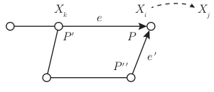
Fig. 1 An example network for EpiHiper with individuals \(P\), \(P'\) and \(P''\). Here, the infectious person P’ may infect the susceptible person \(P\), who as a result may progression from health state \(X\) to an exposed state \(X'\).
shows a network where a susceptible person \(P\) is in contact with infectious persons \(P'\) and \(P''\). Focusing on the the pair \((P',P)\), we combine the {state susceptibility} and {state infectivity} of their respective health states \(X_k\) and \(X_i\) with the {infectivity scaling factor} of \(P'\) and the {susceptibility scaling factor} of \(P\) to form the propensity associated with the contact configuration \(T_{i,j,k} = T(X_i, X_j, X_k)\) for the potential progression of the health state of person \(P\) to \(X_j\) as:
Here, \(T\) is the duration of contact for the edge \(e = (P', P, w, \alpha, T)\), \(w\) is an edge weight, and \(\alpha\) is a Boolean value indicating whether or not the edge is active (e.g., not disabled because of an ongoing school closure).
In the example, there are two transmission configurations (1 susceptible state times 2 infectious states) are
both having the default weight of \(\omega = 1.0\).
Regarding infectivity, people in either of the states \(Isymp\) and \(Iasymp\) can transmit infections, with the asymptomatic reduction in infectivity being 60% and thus \(\beta_\iota(Iasymp) = 0.40\) while the susceptibility and infectivity values of all other health states have the default value of \(1.0\). In addition, the user may define a collection of traits to associate with each edge or node, see Section Traits for full details.
For each time step, and for each person \(P\), the propensities \(\rho\) from (2) are collected across all edges \(e\) and contact configurations T as the sequence \(\rho_P = (\rho(P, P', T, e)_{P', T, e})\). To determine if \(P\) becomes infected is modeled using a Gillespie process [Gil76, Gil77] the person \(P'\) to whom one attributes \(P\) becoming infected is also determined as part of this step.
To determine if an infection takes place, and also to whom we attribute the infection (e.g., \(P'\) or \(P''\) in Fig. 1, we use the Direct Gillespie Method.
Contagion model assumptions. It is assumed that (i) propensities for a person are independent across contact configurations, and (ii) that during any time step no person can change their health state. The first assumption is quite common and not unreasonable for the contact networks that are used. The second assumption can always be accommodated by reducing the size of the time step. Its real purpose is to ensure order invariance of contacts within a time step, thus providing the required guarantee for algorithm correctness.
Parameter
|
Description
|
|---|---|
\(P\), \(P'\)
|
Persons/agents/nodes
|
\(X_i\)
|
Health state \(i\)
|
\(\sigma(X_i)\)
|
Susceptibility of health state \(X_i\)
|
\(\iota(X_i)\)
|
Infectivity of health state \(X_i\)
|
\(\beta_\sigma(P)\)
|
Susceptibility scaling factor for person \(P\)
|
\(\beta_\iota(P)\)
|
Infectivity scaling factor for person \(P\)
|
\(w_e\)
|
Weight of edge \(e = (P, P')\)
|
\(\alpha_e\)
|
Flag indicating whether the edge \(e\) is active
|
\(T(X_i,X_j,X_k)\)
|
Contact configuration for a susceptible progression from \(X_i\) to \(X_j\)
in the presence of state \(X_k\)
|
\(\omega_{i,j,k}\)
|
Transmission weight of contact configuration \(T(X_i, X_j, X_k)\)
|
\(\tau\)
|
Transmissibility
|
\(\rho(P, P', T_{i,j,k},e)\)
|
Contact propensity
|
States
Synopsis
States: a declaration of states of the contagion model
Specification
To define the states of the contagion model, the following syntax is used:
states:       list(state)
state:        id susceptibility infectivity [annotation]
initialState: idRef
Name
|
Type
|
Description
|
|---|---|---|
id
|
An id which has to be unique within the list of states
|
|
susceptibility
|
\(0 \le x \in \mathbb{R}\)
|
The susceptibility of the state
|
infectivity
|
\(0 \le x \in \mathbb{R}\)
|
The infectivity of the state
|
ann:*
|
Optional annotation of the state
|
The idRef property of the initalState must refer to an existing id in the list of the states. The normative JSON schema can be found at: state
Examples
"states": [
  {
    "id": "susceptible",
    "ann:label": "Susceptible",
    "susceptibility": 1.0,
    "infectivity": 0
  },
  {
    "id": "exposed",
    "ann:label": "Exposed",
    "susceptibility": 0,
    "infectivity": 0
  },
  {
    "id": "infectious",
    "ann:label": "Infectious",
    "susceptibility": 0,
    "infectivity": 0.1
  },
  {
    "id": "hospitalized",
    "ann:label": "Hospitalized",
    "susceptibility": 0,
    "infectivity": 0.2
  },
  {
    "id": "funeral",
    "ann:label": "Funeral",
    "susceptibility": 0,
    "infectivity": 0.2
  },
  {
    "id": "removed",
    "ann:label": "Removed",
    "susceptibility": 0,
    "infectivity": 0
  }
],
"initialState": "susceptible",
Progressions
Synopsis
Progressions: the description of all progressions from entry states to exit state, including dwell-time distributions and probabilities.
Specification
To define the progressions between states of the contagion model, the following syntax is used:
transitions:  list(transition)
transition:   id entryState exitState probability dwellTime
              [susceptibilityFactorOperation] [infectivityFactorOperation] [annotation]
Name
|
Type
|
Description
|
|---|---|---|
id
|
An id which has to be unique within the list
of transitions
|
|
entryState
|
idRef
|
The entryState must refer to an existing id in the list
of states.
|
exitState
|
idRef
|
The exitState must refer to an existing id in the list
of states.
|
probability
|
\(0 \le x \in \mathbb{R} \le 1\)
|
The probability that the entry state changes to the
exit state
|
dwellTime
|
The time before the state change occurs
|
|
susceptibilityFactorOperation
|
The numeric operation to be performed on an
individuals susceptibility factor when the
state change occurs
|
|
infectivityFactorOperation
|
The numeric operation to be performed on an
individuals infectivity factor when the
state change occurs
|
|
ann:*
|
Optional annotation of the state
|
If the optional susceptibilityFactorOperation or infectivityFactorOperation are missing no operation will be exectuted, i.e., the current factor will be preserved. The normative JSON schema can be found at: transitions
Examples
"transitions": [
  {
    "id": "exposed2infectious",
    "ann:label": "Exposed->Infectious",
    "entryState": "exposed",
    "exitState": "infectious",
    "probability": 1,
    "dwellTime": {"fixed": 3}
  },
  {
    "id": "infectious2hospitalized",
    "ann:label": "Infectious->Hospitalized",
    "entryState": "infectious",
    "exitState": "hospitalized",
    "probability": 0.1111,
    "dwellTime": {"fixed": 2}
  },
  {
    "id": "infectious2funeral",
    "ann:label": "Infectious->Funeral",
    "entryState": "infectious",
    "exitState": "funeral",
    "probability": 0.6667,
    "dwellTime": {"fixed": 10}
  },
  {
    "id": "infectious2removed",
    "ann:label": "Infectious->Removed",
    "entryState": "infectious",
    "exitState": "removed",
    "probability": 0.2222,
    "dwellTime": {"fixed": 12}
  },
  {
    "id": "hospitalized2funeral",
    "ann:label": "Hospitalized->Funeral",
    "entryState": "hospitalized",
    "exitState": "funeral",
    "probability": 0.1111,
    "dwellTime": {"fixed": 15}
  },
  {
    "id": "hospitalized2removed",
    "ann:label": "Hospitalized->Removed",
    "entryState": "hospitalized",
    "exitState": "removed",
    "probability": 0.8889,
    "dwellTime": {"fixed": 15}
  },
  {
    "id": "funeral2removed",
    "ann:slabel": "Funeral->Removed",
    "entryState": "funeral",
    "exitState": "removed",
    "probability": 1,
    "dwellTime": {"fixed": 1}
  }
]
Transmissions
Synopsis
Transmissions: the description of the contact configurations \(T(X_i, X_j, X_k)\) for individuals causing a state change.
Specification
To define possible transmission between occurring between individuals in the contagion model, the following syntax is used:
transmissions:    list(transmission) [transmissibility]
transmission:     id entryState exitState probability transmissibility
                  [susceptibilityFactorOperation] [infectivityFactorOperation] [annotation]
transmissibility: x >= 0
Name
|
Type
|
Description
|
|---|---|---|
id
|
An id which has to be unique within the list
of transmissions
|
|
entryState
|
idRef
|
The entryState must refer to an existing id in the list
of states.
|
exitState
|
idRef
|
The exitState must refer to an existing id in the list
of states.
|
contactState
|
idRef
|
The contactState must refer to an existing id in the list
of states.
|
transmissibility
|
\(0 \le x \in \mathbb{R}\)
|
The transmissibility of the for each contact.
|
susceptibilityFactorOperation
|
The numeric operation to be performed on an
individuals susceptibility factor when the
state change occurs
|
|
infectivityFactorOperation
|
The numeric operation to be performed on an
individuals infectivity factor when the
state change occurs
|
|
ann:*
|
Optional annotation of the state
|
If the optional susceptibilityFactorOperation or infectivityFactorOperation are missing no operation will be executed, i.e., the current factor will be preserved. The normative JSON schema can be found at: transmissions. The optional model attribute transmissibility is used to scale all individual transmissibilities. Its default value is \(1.0\)
Examples
"transmissions": [
  {
    "id": "contactWithInfectious",
    "ann:label": "Susceptible -> Exposed {Infectious}",
    "entryState": "susceptible",
    "exitState": "exposed",
    "contactState": "infectious",
    "transmissibility": 1
  },
  {
    "id": "contactWithHospitalized",
    "ann:label": "Susceptible -> Exposed {Hospitalized}",
    "entryState": "susceptible",
    "exitState": "exposed",
    "contactState": "hospitalized",
    "transmissibility": 1
  },
  {
    "id": "contactWithFuneral",
    "ann:label": "Susceptible -> Exposed {Funeral}",
    "entryState": "susceptible",
    "exitState": "exposed",
    "contactState": "funeral",
    "transmissibility": 1
  }
],
"transmissibility": 0.8
Bibliography
D.T. Gillespie. A general method for numerically simulating the stochastic time evolution of couple chemical reactions. Journal of Computational Physics, 22:403–434, 1976.
Daniel T. Gillespie. Exact stochastic simulation of coupled chemical reacitions. Journal of Physical Chemistry, 81(25):2340–2361, 1977.